 |
 |
Investment is the act of acquiring income-producing assets, known as physical capital, either as additions to existing assets or to replace assets that have worn out (depreciated). These assets may be in the form of fixed nonresidential plant and equipment, housing (fixed residential) or business inventories. Decisions about the appropriate quantity of assets or capital are often based on profit-maximizing behavior of a private business firm producing goods and services or providing housing services.
The investment relationship may be written as follows:
Jt = K*t - Kt-1 + δKt-1
where
The difference in the first two terms ( K*t - Kt-1 ) represents net or new investment and the last term (δ Kt-1) represents replacement investment. Gross investment is just the sum of the two expressions.
By multiplying both sides of the equation by Pk (the price of capital) and factoring out ' Kt-1', we can write an expression for Investment expenditure(It):
It = Pk[K*t - (1-δ)Kt-1]
where
It = PkJt.
The key to understanding investment decisions is the determination of K*, the desired capital stock. This desired level is based, as stated above, on profit-maximizing behavior of the firm. There are several methods by which we can approach the profit-maximizing level of capital stock. First, we can analyze the net present value of different amounts of capital to determine which quantity gives the greatest discounted stream of profits. For example, given the following:
With this data we will use the following annuity factor computation:
PVn = (Revenue)[1 - (1+r)-n] / r
= (Revenue)[1 - (1.05)-10] / 0.05 = (Revenue)7.722
K Output
(units)Revenue PV
(n=10)less Costs
[Pk(K)]Net Present Value 1 50 $250 $1930.50 $1000 $930.50 2 90 $450 $3474.90 $2000 $1474.90 3 120 $600 $4632.00 $3000 $1632.00 4 140 $700 $5405.40 $4000 $1405.40 5 150 $750 $5791.50 $5000 $791.50
In the above example (assuming diminishing marginal productivity) we find that three units of capital would generate the greatest net present value and thus the greatest profits.
A second approach is the marginal approach where we compare the contribution to revenue by using one more unit of capital with the costs of acquiring that unit of capital. The contribution to revenue is known as the Marginal Revenue Product (MRP) of capital and is calculated by multiplying the marginal product with the market price of the output produced:
MRPk = MPKPx
The contribution to costs is known as the Rental Cost of Capital (RCC) which includes borrowing costs (or opportunity costs of using internal funds for investment expenditure) and depreciation costs:
RCC =PK(r) + PK( δ ) = PK(r + δ )
We will use similar data and a table for an example:
| K | Output | MPk | MRPk | RCC (r = 5%, δ = 10%) |
| 1 | 50 units | 50 | $250 | $150 |
| 2 | 90 | 40 | $200 | $150 |
| 3 | 120 | 30 | $150 | $150 |
| 4 | 140 | 20 | $100 | $150 |
| 5 | 150 | 10 | $50 | $150 |
If the MRP exceeds RCC then profits will increase by acquiring additional units of capital (contribution to revenue exceed contribution to costs). If the opposite is true then the additional costs associated with one more unit of capital exceed the revenue generated and profits will decline.
Similar to the Net Present Value approach, we find that with three units of capital the contribution to revenue of the third unit is just equal to the costs of acquiring and using that third unit--profits will be a maximum at this level of input as shown in the diagram below-left.
|
|
A change in interest rates would increase the rental cost of capital 'RCC' such that this third unit is no longer profitable. The firm would react to this cost increase (an increase in the price of capital would have similar effect), by using less capital in production. This is shown in the above diagram-right.
A third approach is using a calculation similar to the present value of a perpetuity (again, see the. We begin by using the marginal conditions above:
Marginal Revenue Product = Rental Cost of Capital
MPKPx = PK(r + δ)
And we rearrange the terms:
[MRPK - PK (δ )] / PK = ' θ '
This term θ represents the yield on the last unit of capital employed in the production process:
| K | Output | MRPK - PK (δ ) | PK | Yield |
| 1 | 50 units | $250-$100 | $1000 | 15% |
| 2 | 90 | $200-$100 | $1000 | 10% |
| 3 | 120 | $150-$100 | $1000 | 5% |
| 4 | 140 | $100-$100 | $1000 | 0% |
| 5 | 150 | $50-$100 | $1000 | NA |
In this case, we find that the yield on the first two units of capital is greater than the market interest rate and thus may be acquired to earn profits over-and-above the borrowing costs. It is the third unit of capital where the yield is just equal to the market rate of interest -- no additional profits may be earned by hiring additional capital.
In all three approaches we find that the desired capital stock 'K*' is equal to three units based on the productivity of capital, the rate of depreciation, the price of capital and the output being produced and, of greatest importance, market interest rates.
We can use a Cobb-Douglas form of the production function to solve for K* and combine this with the expression for investment defined above:
Xoutput = AL α K β and MPk = β X/K
given MRPk = RCC,
β (X/K)Px = Pk(r+ δ )
or
K* = [ β (Px)X] / [Pk(r+ δ )]
Inserting this expression for K* into the investment expenditure equation gives us:
It = Pk{ [β (Px)X] / [Pk(r+ δ )] - (1- δ)Kt-1}
or
It = [ β (Px)X] / (r+ δ ) - (1- δ)PkKt-1
where we find that Investment is inversely related to market interest rates and the price of a unit of capital, positively related to output prices and the productivity of capital (as measured by the parameter ' β, and undetermined with respect to the rate of depreciation.
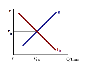
The Supply of Loanable Funds 'S' is commonly upward sloping -- a positive relationship between savings and the real interest rate 'r'. This willl hold true as long as the substitution effect is stronger than the income effect. The Demand for Loanable Funds I0 -- investment expenditure is inversely related to real interest rate 'r' as a higher rental cost of capital will lead to a smaller optimal capital stock.
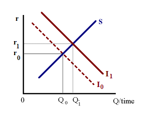
Combining the two relationships, we find an equilibrium interest rate at r0 where savings is equal to investment expenditure -- shown on figure 2 left. With an increase in the optimal capital stock and corresponding increase in investment demand, we find the demand for funds shifting outward to I1. With an upward sloping supply of funds, this leads to an increase in the real interest rate r and an increase in the quantity of funds traded -- shown on figure 2 right.
|
|