| . |
© 1999-2002
Douglas A.Ruby
Aggregate Demand
Aggregate Expenditure
Money Demand
Macroeconomics
|
Demand-Side Equilibrium
Equilibrium in Financial Markets (version I)
A standard expression for money demand (as derived from the Inventory
Theoretic Model) is:
Md* = Z(Y)r /
(i)b
where the exponents represent the sensitivity of money demand to income 'Y'
and nominal interest rates 'i'.
If we solve for 'i' in this expression, we have:
i = [ZYr / Md]
1/b
In equilibrium Md = Ms or:
Md = M/P
where M/P represents the purchasing power of available money
balances (the money supply). Holding the price level constant (no supply-side constraints),
changes in purchasing power
will only result via changes in the money supply. Additionally, if the
price level is unchanging then nominal measures of income are the same as
real income measures.
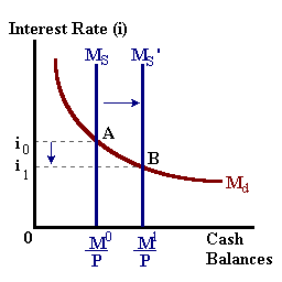
figure 1
An increase in the Money Supply |
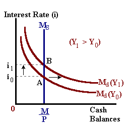
figure 2
An increase in Income 'Y' and Md |

|

|
| An increase in the Money Supply (Real money balances) shifts
the this function to the right. This is often a deliberate policy action (via open-market operations)
usually intended to
stimulate aggregate demand. The result is an Excess Supply
of Money (specifically excess and loanable reserves) such that interest rates fall. |
An increase in Income 'Y' leads to an outward shift
in Money Demand (due the the need to support a greater level of
transactions). This shift leads to an Excess Demand for Money where individuals
will begin to make portfolio adjustments (selling bonds and securities thus Pbonds
decline, Ybonds
increase) thus pushing
interest rates up. |
Substituting in the above equation, we have
i = [(Z)(P)(Y)a / M]
1/b
This is an expression for equilibrium in money or financial markets in
the aggregate economy known and the
LM (Liquidity demand = Money supplied) Curve.
In this expression the equilibrium interest rate and income are directly
related.
If the price level (and hence the rate of inflation
'p is held constant then the
nominal interest rate 'i' is identical to the real interest rate 'r'
allowing
LM = {Y, r
e R2 |
M = Z(P)(Y)r/(r)b
}
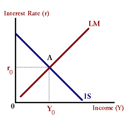
Putting the two expressions together, we can determine a level of
income 'Y' and interest rate 'r' such that both Product Markets and
Financial Markets are in equilibrium.

Reset
IS
LM
Increases in autonomous spending Ao (i.e. an increase in Government
spending) would lead
to an outward shift on the IS curve and
a corresponding increase in both the level of income and interest rates
(Press the IS button).
Increases in the money supply 'M/P' would shift the
LM curve downward with a resulting decrease in interest rates and
and increase in income (Press the LM button).
|